导图社区 Reading 6- organizing, visualising, and describing data
Reading 6- organizing, visualising, and describing data
这是一篇关于Reading 6- organizing, visualising, and describing data的思维导图。
编辑于2022-06-07 11:45:04- CFA I - Quantitative
- 相似推荐
- 大纲
导图社区 Reading 6- organizing, visualising, and describing data
这是一篇关于Reading 6- organizing, visualising, and describing data的思维导图。
编辑于2022-06-07 11:45:04