导图社区 2.2 Aggregate demand and Aggregate supply IBDP economics
- 29
- 0
- 0
- 举报
2.2 Aggregate demand and Aggregate supply IBDP economics
Aggregate demand and Aggregate supply IBDP economics:Aggregate demand (AD)、Aggregate Supply (AS).
编辑于2022-06-01 00:49:41- Economic…
- Aggregate
- 相似推荐
- 大纲
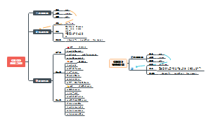
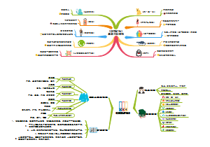
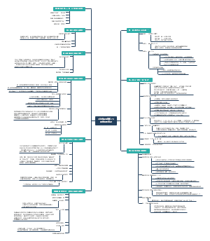

2.2 Aggregate demand and Aggregate supply
Aggregate demand (AD)
An ⇧ in AD ⇨ shift to right, from AD1 to AD2
An ⇩ in AD ⇨ shift to left, from AD1 to AD3
Difference between micro demand and macro AD
Micro demand (D)= quantity of a single product that consumers are willing and able to buy at different prices, over a specific time period, ceteries paribus.
negative relationship between price and quantity is due to diminishing marginal benefits
Macro aggregate demand (AD)= total quantity of aggregate output, or real GDP, that all buyers (consumers, firms, government, and foreigners) in an economy want to buy at different possible price levels, in a year, ceteris paribus.
negative slope (downward sloping), indicating a negative relationship between the price level and real output, or GDP
AD curve has a negative slope
wealth effect (weath= value of all assets owned, including property, savings, stocks, bonds, etc)
If price level ↑ ➔ real value of wealth ↓ ➔ people feel poorer ➔ spending on output↓ ➔ upward movement along the AD curve
interest rate effect
If price level ↑ ➔ consumers and firms need more money for their transactions ➔ demand for money↑ ➔ interest rate↑ ➔ cost of burrowing↑ ➔ consumer and firm spending↓ ➔ ∵ lower borrowing ➔ there is an upward movement along the AD curve
international trade effect
If price level↑ ➔ exports become more expensive to foreigners ➔ quantity of exports(X) demanded by foreigners↓
Imports(M) become relatively cheaper to domestic residents ➔ quantity of imports↑ ➔ (X-M)↓ ➔ there is an upward movement along the AD curve
Determinants of AD (causes of AD shifts)
Consumption
Inventment
Government Spending
Net Export
AD increases, shifting to the right, when
Consumption spending↑, when
Consumer confidence↑ ➔ consumers become more optimistic about the future of the economy
Interest rates↓ ➔ costs of borrowing↓ ➔ consumer borrowing↑ (expansionary monetary policy)
Wealth↑ (ex. stock market or house prices rise) ➔ consumers feel wealthier
Personal income taxes↓ ➔ disposable income↑ (expansionary fiscal policy, or market-based supply-side policy)
househould indebtedness (debt)↓ ➔ consumers feel more comfortable about their spending
Investment spending↑, when
business confidence↑ ➔ firms becomre more optimistic about the future of the economy
interest rate↓ ➔ cost of borrowing↓ ➔ firm borrowing↑ (expansionary policy)
technological improvements ➔ investment spending↑
business taxes↓ ➔ after-tax profits↑ (expansionary fiscal policy)
corporate indebtedness (debt) ↓ ➔ firms feel more comfortable about investment spending
Government spending↑, when
political priorities of the government change ➔ spending on various activities↑ (ex. education, health care, infrastructure, defense...)
economic priorities ➔ government↑ spending on various activities (expansionary fiscal policy, or interventionist supply-side policy)
Net export(X-M)↑, when
income of trading partners abroad↑ ➔ demand for a country's exports↑
a country's exchange rate↓ ➔ exports become cheaper to foreigners and imports become more expensive to domestic residents ➔ exports↑ & imports↓ ➔ net exports (=X-M)↑
trade protection abroad↓ (=fewer restrictions on imports in other countries)➔ a country's exports↑
domestic trade protection↑ (=more restrictions on imports from other countries) ➔ import↓ ➔ net exports↑
AD decrease, shifting to the left, when
Consumption spending↓
Inveestment spending↓
Government spending↓
Net export(X-M)↓
Aggregate Supply (AS)
An ⇧ in SRAS ⇨ right: SRAS1⟹SRAS2
A⇩ in SRAS ⇨ left: SRAS1⟹SRAS3
Aggregate supply (AS)= total quantity of goods and services produced in an economy (real GDP) over a particular time period at different price levels.
Short run = the period of time when all resource prices (wages and prices of all other factors of production) are constant
Long run = period of time when all resource prices (wages and prices of all factors of production) change to match changes in the price level
Long-run aggregate supply (LRAS)
Keynesian AS
Short-run aggregate supply
AS curve has an upward slope: there's a positive relationship between the price level and real GDP
Firm profitability: If price level↑ (with wages and all other factor prices held constant) ➔ firms' profits increase ➔ firms ↑ quantity of output they produce ➔ upward movement along the SRAS curve
price level↓ ➔ firms' profits fall ➔ firms decrease the quantity of output they produce ➔ downward movement along SRAS curve
Changes in SRAS (shifts)
Factors causing SRAS↑, shifting right
↓ in resource prices ➔ costs of production↓
↓ in business taxes
↑ in subsidies
positive supply shock ➔ agricultural output↑
Factors causing SRAS↓, shifting left
Equilibrium in short run and changed in short run equilibrium`
intersection of AD and SRAS determines short-run equilibrium in the economy, indicating equilibrium real output (real GDP)
Changing short-run equilibrium due to changes in AD
As AD↑ ➔ price level↑ and real GDP↑
As AD↓ ➔ price level↓ and real GDP↓
Changing short-run equilibrium due to changes in SRAS
As SRAS↑ ➔ price level↓ and real GDP↑
As SRAS↓ ➔ price level↑ and real GDP↓
Monetarist/new classical model based on the assumption that when product and resource markets are free to work competitively according to demand and supply, product prices and resource prices will be flexible in the upward and downward directions, and the economy will be able to move into the long run, where resource prices change to match changes in price level
Long-run aggregate supply (LRAS)
full employment output= potential output= output where cyclical umemployment is 0, unemployment=natural rate
LRAS is verticle because in long-run, resource prices change along with the price level, therefore in real terms resource prices remain constant. Thus, as price level increase or decrease, firm profitability is constant, and firm face no incentive to change the quantity of output they produce.
quantity pf output produced in the long run is independent of the price level
Long-run equilibrium in the monetarist/new classical model
Long-run equilibrium occurs at the level of potential output, Yp, or full unemployment output, where AD and SRAS intersect on the LRAS curve
Inflationary and deflationary (recessionary) gaps
Deflationary (=recessionary) gap: short-run equilibrium (Ye) < potential GDP (Yp)
Deflationary gap occurs when short-run equilibrium GDP (Ye) < potential GDP (Yp) due to insufficient AD.
A deflationary gap can only persist in the short-run. In the long-run, the economy will return to potential output
Suppose the economy is initially at point a at long-run equilibrium producing Yp. Due to a decrease in AD (AD1 to AD2) it moves to point b where the price level has fallen, real GDP s lower at Ye and there is a deflationary gap. The economy can remain at b only in the short run. In the long-run, wages and other resource prices will fall to match the fall in price level ➔ SRAS↑
In the long run, the only effect of a fall in AD is to cause a fall in the price level, with no effect on real GDP
Inflationary gap: short-run equilibrium (Ye) > potenial GDP(Yp)
Due to excess aggregate demand
Suppose the economy is initially at point a at the LR equilibrium producing output Yp. Due to an increase in AD, it moves to point b, where the PL is higher, real GDP is greater at Ye, and there's an inflationary gap (only in a short run). In the long run, wages and other resource prices rise to match the increase in PL ➔ SRAS decreases.
In the long run, only effect of an increase in AD is to cause an increase in PL, no effect on real GDP
In the monetary/new-classical model, fluctuations of output occur only in the short run. In the long run, the economy automatically returns to long-run equilibrium and full employment (potential) output because of the assumption of full wage-price flexibility. Therefore, long-run equilibrium occurs at full employment output.
Change in long-run equilibrium
with a constant LRAS and potential output, leading to changes only in the price level
with a changing LRAS, leading to increasing potential output (economic growth) or decreasing output (negative growth)
Keynesian model: there is no long run, because wages (and other resource prices) as well as the price level do not fall easily.
i. horizontal section
wage-price downward inflexibility: wages do not fall easily because of wage contracts, minimun wages, and inpopularity of wage cuts.
if wages do not fall, a drop in product prices would cut into firms' profits, which firms wish to avoid
spare capacity when the economy is in recession: A low levels of output, when the economy is in recession, there's unemployment of labor and other resources, so if firms decide to increase output and demand more resources, there's no upward pressure on wages and the price level, therefore they do not increase.
ii. upward sloping section
resource bottlenecks (shortage) that appear as output increases and approaches full employment or potential output (Yp), causing resource prices to increase.
As firms' costs of production ↑, firms↑ product prices so the price level begins to rise.
iii. vertical section
maximun capacity output (Ym) is reached. all resources are employed to their maximun extent, and is therefore not possible for output to increase turther.
Any effort to increase output beyond this point results only in increases in the price level
Equilibrium in the Keynesian model
Equilibrium GDP (Ye) < Potential GDP (Yp)
Equilibrium GDP (Ye) > Potential GDP(Yp)
potential output (Yp) is reached
Shifts in AS over the long term and economic growth
Increase in quantity of factos of production
Increase in quality of factors of production
technological changes which could involve improvements in the quality of capital goods
reductions in the natural rates of unemployment
improvements in efficiency
institutional changes