导图社区 Econometrics
- 57
- 0
- 0
- 举报
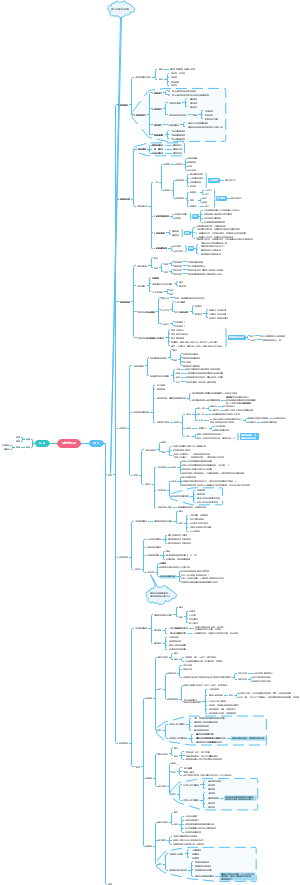
Econometrics
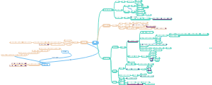
Econometrics Chapter 1 The Nature of Econometrics and Economics Data Chapter 2 The Simple Regression Model Chapter 3 Multiple Regression Analysis :Estimation Chapter 4 Multiple Regression Analysis :Inference Chapter 6 Multiple Regression Analysis :Further Issues Chapter 7 Multiple Regression Analysis with Qualitative Information Chapter 8 Heteroskedasticity Chapter 10 Basic Regression Analysis with Time Series Data Chapter 12 Serial Correlation and Heteroskedasticity in Time Seri
编辑于2023-04-06 16:40:46 甘肃- Econometrics 计量经济学
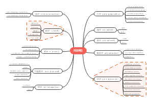
- 企业产出统计
关于企业产出统计的思维导图,整理了总产值、增加值、生产净值的知识点,大家可以学起来哦。
- 财经应用文写作
财经应用文,广义指党政机关、社会团体、企事业单位等各种法定的社会组织在处理公务过程中形成并使用的文字材料;狭义指党政机关实施领导、履行职能、处理公务的具有特定效力和规范体式的文书。
- Econometrics
Econometrics的思维导图,分别有: Chapter 1 The Nature of Econometrics and Economics Data Chapter 2 The Simple Regression Model Chapter 3 Multiple Regression Analysis :Estimation Chapter 4 Multiple Regression Analysis :Inference Chapter 6 Multiple Regression Analysis :Further Issues Chapter 7 Multiple Regression Analysis with Qualitative Information Chapter 8 Heteroskedasticity Chapter 10 Basic Regression Analysis with Time Series Data Chapter 12 Serial Correlation and Heteroskedasticity in T
Econometrics
社区模板帮助中心,点此进入>>
- 企业产出统计
关于企业产出统计的思维导图,整理了总产值、增加值、生产净值的知识点,大家可以学起来哦。
- 财经应用文写作
财经应用文,广义指党政机关、社会团体、企事业单位等各种法定的社会组织在处理公务过程中形成并使用的文字材料;狭义指党政机关实施领导、履行职能、处理公务的具有特定效力和规范体式的文书。
- Econometrics
Econometrics的思维导图,分别有: Chapter 1 The Nature of Econometrics and Economics Data Chapter 2 The Simple Regression Model Chapter 3 Multiple Regression Analysis :Estimation Chapter 4 Multiple Regression Analysis :Inference Chapter 6 Multiple Regression Analysis :Further Issues Chapter 7 Multiple Regression Analysis with Qualitative Information Chapter 8 Heteroskedasticity Chapter 10 Basic Regression Analysis with Time Series Data Chapter 12 Serial Correlation and Heteroskedasticity in T
- 相似推荐
- 大纲
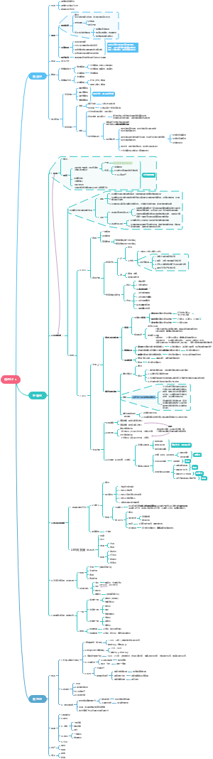
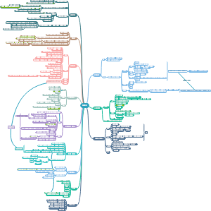
Econometrics
Chapter 1 The Nature of Econometrics and Economics Data
Definition of Econometrics
use of statistical methods to analyze economic data
data form
experimental data
nonexperimental data
Econometrics typically analyze
Typical goals of econometrics analysis
Estimating relationship between economic variables
Testing economic theories and hypotheses
Forecasting economic variables
Evaluating and implementing government and business policy
"ETFE "
Steps in econometric analysis
Economic model (this step is often skipped )
Maybe micro-or macromodels
Often use optimizing behavior,equilibrium modeling,...
Establish relationships between economic variables
Example :demand equation,pricing equation,...
理论模型,是一种函数关系
Functional form of relationship not specified
Equation could have been postulated without economic modeling
Econometric model
计量模型,是一种相关关系
The functional form has to be specified
Variable may have to be approximated by other quantities
Most of econometrics deals with the specification of the error
May be used for hypothesis testing
Econometrics analysis
Requires economic data
Cross-sectional data 随机抽样而来,离散性高
Sample of individuals,households,firms cities,states,countries,or other units of interest at a given point of time /in a given period
Cross-sectional observations are more or less independent
Sometimes pure random sampling is violated,e.g.units refuse to respond in surveys,or if sampling is characterized by clustering
Cross-sectional data typically encountered in applied microeconomics
For example,pure random sampling from a population
Time series data
Observations of a variable or several variables over time
Time series observations are typically serially correlated
Ordering of observations conveys important information
Data frequency:daily,weekly,monthly,quarterly.,annually,….
Typical features of time series:trends and seasonality
Typical applications:applied macroeconomics and finance
For example,stock prices,money supply,consumer price index, gross domestic product,annual homicide rates,automobile sales,..
Pooled cross data
Two or more cross sections are combined in one data set
Cross sections are drawn independently of each other
Pooled cross sections often used to evaluate policy changes
Example
Random sample of house prices for the year 1993
Evaluate effect of change in property taxes on house prices
A new random sample of house prices for the year 1995
Compare before/after (1993:before reform,1995:after reform)
Panel /Longitudinal data
The same cross-sectional units are followed over time
Panel data have a cross-sectional and a time series dimension
Panel data can be used to account for time-invariant unobservables
Panel data can be used to model lagged responses
Example
City crime statistics;each city is observed in two years
Time-invariant unobserved city characteristics may be modeled
Effect of police on crime rates may exhibit time lag
Causality and the notion of ceteris paribus
Definition of causal effect of x on y:
"How does variable y change if variable x is changed but all other relevant factors are held constant"
Most economic question are ceteris paribus question
It is important to define which causal effect one is interested in
It is useful to describe how an experiment would have to be designed to infer the causal effect in question
Chapter 2 The Simple Regression Model
Definition
Explains of the simple linear regression model
y:explained variable
βο:intercept
β1:slope parameter
x:explained variable
u:error term
interpretation
△y/△x=β1
△u/△x=0
Conditional mean independence assumption
E(u|x)=0
The explanatory variable must not contain information about the mean of the unobserved factors
Population regression function (PFR)
x变动一个单位,y的条件期望变动β1个单位
y为正态分布——>u为正态分布
大多数数据分布在均值附近,所以抽样数据更具有代表性
Ordinary Least Squares(OLS) estimates
β1(hat)的大小与x,y间的相关性没有联系
线在点中间
E(u|x)=0
回归线在点中间
Fitted values and residuals
Algebraic properties of OLS regression
Deviations from regression line sum up to zero
Covariance between deviations and regressions is zero
Sample averages of y and x lie on regression line
Goodness-of-fit
Measures of Variation
离差(Total variation )
回归平方和(Explained part )
残差平方和(Unexplained part )
SST=SSE+SSR
Measure
R-squared (拟合优度/判定系数/决定系数)
R-squared越大,拟合地越好
R-squared 不是判定模型是否有用的依据
A high R-squared does not necessarily mean that the regression has a causal interpretation !
Expected values and variances of the OLS estimators
Unbiasedness of OLS
SST 越大,估计区间越小,估计就越准确,因此SST 不能等于0
Variances of the OLS estimators
Standard assumptions for the linear regression model
Assumption SLR.1
Linear in parameters
In the population,the relationship between y and x is linear
Assumption SLR.2
Random sampling
The data is random sample drawn from the population
简单随机抽样
分层抽样
系统抽样
整群抽样
Each data point therefore follows the population equation
Assumption SLR.3
Sample variation in the explanatory variable
The values of the explanatory variables are not all the same
Assumption SLR.4
Zero conditional mean
The value of the explanatory variable must contain no information about the mean of the unobserved factors
Theorem2.1
Assumption SLR.5
Homoskedasticity
The value of the explanatory variable must contain no information about the variability of the unobserved factors
Theorem 2.2
Incorporating nonlinearities
Logarithmic form
Log-logarithmic form
当x增加量改变1%时,歪的增加量改变△log(y)/y%个单位
Logarithmic changes are always percentage changes
The log-log form postulates a constant elasticity model
Estimating the error variance
standard errors
Chapter 3 Multiple Regression Analysis :Estimation
Definition
Explain variable y in terms of variables x 1,x 2,…x k
β1:除了x1以外,其他变量都不变时x1对y的影响
β1等
simple:直接+间接影响
multiple:直接影响
当simple与multiple中的β1相等时,r(x1,xi)=0
解释变量:k个,参数:k+1个
β1…βk
simple:回归系数
multiple:偏回归系数(partial)
不能凭借β间的大小来判断解释变量对被解释变量的影响程度
因为解释变量间的数量级不同
当其他参数和误差项保持不变时,第j个解释变量xj变动一个单位,y变动βj个单位
Motivation for multiple regression
Incorporate more explanatory factors into the model
Explicitly hold fixed other factors that otherwise would be in u
Allow for more flexible functional forms
Multivariate model
二元(three-variable model)
k元(k+1-variable model)
OLS Estimation
Fitted values and residuals
Algebraic properties of OLS regression
Why does this procedure work ?
The residuals from the first regression is the part of the explanatory variable that is uncorrelated with the other explanatory variables
The slope coefficient of the second regression therefore represents the isolated effect of the explanatory variable on the dep. variable
Goodness-of-Fit
R-squared
Expected values and variances of the OLS estimators
Unbiasedness of OLS
1/(1-R^2)叫做VIF (方差膨胀因子)
VIF 越大,共线性越严重
0<VIF <10,不存在多重共线性
VIF ≥10(R^2≥0.9),存在多重共线性
VIFj =1/(1-Rj^2)
Rj^2:用其他变量解释xj时的R^2
Conclusion :x之间最好不相关
Sampling variances of the OLS slope estimators
Standard assumptions for the multiple regression model
Assumption MLR.1(经典线性模型假定)
Linear in parameters
Assumption MLR.2
Random sampling
Assumption MLR.3
No perfect collinearity
In the sample (and therefore in the population), none of the independent variables is constant and there are no exact linear relationships among the independent variables
Imperfect correlation is allowed
If an explanatory variable is a perfect linear combination of other explanatory variables it is superfluous(多余的) and may be eliminated(消除)
Constant variables are also ruled out(排除) (collinear with intercept)
若存在共线,可增加样本量来调整
Assumption MLR.4
Zero conditional mean
In a multiple regression model, the zero conditional mean assumption is much more likely to hold because fewer things end up in the error
Theorem 3.1
Assumption MLR.5
Homoskedasticity
不会有偏误
Theorem 3.2
Gauss-Makov Theory
BLUEs
Theorem 3.4
The variable problem of regression model
including irrelevant variables in a regression model
omitting(漏掉) relevant variables
影响更大
All estimated coefficients will be biased
When is there no omitted variable bias
If the omitted variable is irrelevant or uncorrelated
Discussion of the multicollinearity problem
lump (合并为一个)
because effects cannot be disentangled(分清)
drop (删掉剩一个)
may reduce multicollineariy(but this may lead to omitted variable bias )
Estimating the error variance
Theorem 3.3
Unbiased estimated of the error variance
Variances in misspecified models
It might be the case that the likely omitted variable bias in the misspecified model 2 is overcompensated by a smaller variance
Conditional on x1 and x2, the variance in model 2 is always smaller than that in model 1
Do no include irrelevant regressors
Trade off bias and variance.bias will not vanish even in large samples
Estimating of the sampling variance of the OLS estimators
sd :观测值的方差
se:估计量的方差
Chapter 4 Multiple Regression Analysis :Inference
Statistical inference in the regression model
Hypothesis tests about population parameters
Construction of confidence intervals
Sampling distributions of the OLS estimators
We already know their expected values and their variances
However, for hypothesis tests we need to know their distribution
In order to derive their distribution we need additional assumptions
Assumption about distribution of errors: normal distribution
Assumption MLR.6 Normality of error terms
Theorem 4.1&4.2
4.1 Normal sampling distributions
4.2 t-distribution for the standardized estimators
The t-distribution is close to the standard normal distribution if n-k-1 is large
independently of xi1,xi2,…,xik
testing
Hо:怀疑结果(大概率事件) H1:样本呈现结果(小概率事件)
t-test
检验对单个总体参数的假设(检验变量的有效性,临界值为2)
testing hypotheses about a single population parameter
Hо:βj=0
t-statistic(t-ratio )
Rejection region
one-sided
two- sided
Confidence intervals
左C0.05:Lower bound of the Confidence interval
右C0.05:Upper bound of the Confidence interval
0.95:Confidence level
Statistically significant
|t-ratio |>1.645
statistically significant at 10% level
|t-ratio |>1.96
statistically significant at 5% level
|t-ratio |>2.576
statistically significant at 1% level
testing more general hypotheses
Hо:βj=aj
t-statistic
用t检验删无关变量前提
数据充分,可靠
Testing hypotheses about a linear combination of the parameters
Define θ1=β1-β2 and test Hо:θ1=0 against H1:θ1<0
F-test
对多个线性约束的检验(检验模型的有效性,临界值为4)
Testing multiple linear restrictions
q:number of restrictions
Example
Hо:β3=0,β4=0,β5=0 against H1:Hо is not true
若Hо成立,责二元和五元无差别
The likely reason is multicollinearity between them
Rejection region
Testing of overall significance
The test of overall significance is reported in most regression packages; the null hypothesis is usually overwhelmingly rejected
The F-testworks for general multiple linear hypotheses
For all tests and confidence intervals, validity of assumptions MLR.1 – MLR.6 has been assumed
Chapter 6 Multiple Regression Analysis :Further Issues
More on using logarithmic functional forms
positive
Convenient percentage/elasticity interpretation
Slope coefficients of logged variables are invariant to rescalings (缩小尺度)
Taking logs often eliminates /mitigates problems with outliers (异常值)
Taking logs often helps to secure normality and homoskedasticity
drawback
Variables measured in units such as years should not be logged
Variables measured in percentage points should also not be logged
Logs must not be used if variables take on zero or negative values
It is hard to reverse(还原) the log-operation when constructing predictions
More on Functional Form
Logarithmic functional forms
Quadratic functional forms
Models with interaction terms
β2:Effect of x2,but for x1 of zero
so interaction effects complicate interpretation of parameters
Reparametrization of interaction effects
δ2:effect of x2 if all variables take on their mean values
μ1.μ2:population means ;may be replaced by sample means
advantages
Easy interaction of all parameters
Standard errors for partial effects at the mean values available
If nnecessary interaction may be centered at other interesting values
General remarks on R-squared
A high R-squared does not imply that there is a causal interpretation
A low R-squared does not preclude precise estimation of partial effects
Adjusted R-squared
punishment :k越大,R^2越小
Adjusted R-squared 比较条件
相同变量
多元模型
当adjusted R-squared <0时,将其看做等于零,即拟合程度差
Nonnested model
In the given example,even after adjusting for the difference in degree of freedom,the quadratic model is preferred
Adding regressors to reduce the error variance
may excarcerbate(排除) multicillinearity problem
reduce the error variance
Variables that are uncorrelated with other regressors should be added because they reduce error variance without increasing multicollinearity
However,such uncorrelated variables may be hard to find
Chapter 7 Multiple Regression Analysis with Qualitative Information
Qualitative Information
A way to incorporate qualitative information is to use dummy variables
They may appear as the dependent or as independent variables
A single dummy independent variable
example
δо=0:基准(bench mark)男性
δ0<0:其他不变时,wage女性<男性
当female=1时,截距为βо+δо
当female=0时,截距为βо
Using dummy explanatory variables in equations for log(y)
当x4变动一个单位时,y改变a%
Dummy variances
Dummy variable trap
single category
某一定性变量有k个分类时,应选k-1个哑变量
multiple categories
用途
政策评价
政策评估
模型比较
Interaction involving dummy variables
改变Slope(有交互项) 还是Intercept (有哑变量) ?
都引入方程进行t检验判断
example
Hypotheses
Hо:δ1=0
The return to education is the same for men and women
Hо:δо=0,δ1=0
The whole wage equation is the same for men and women
Conclusion
No evidence against hypothesis that the return to education is the same for men and women
the effect for educ = 0
模型比较
F检验
The linear probability model
Disadvantages
Predictedprobabilities may be larger than one or smaller than zero
Marginal probability effects sometimes logically impossible.
The linear probability model is necessarily heteroskedastic
Heteroskedasticity consistent standard errors need to be computed
Advantages
Easy estimation and interpretation
Estimated effects and predictions are often reasonably good in practice
Chapter 8 Heteroskedasticity
指回归规模型中扰动项的方差不全相等,即随机扰动项不再是一个常数
Consequences of heteroskedasticity for OLS
OLS still unbiased and consistent under heteroskedasticity (有效性??)
interpretation of R-squared is not changed
invalidates variance formulas for OLS estimators
The usual F tests and t tests are not valid
OLS is no longer the best linear unbiased estimator (BLUE )there may be more efficient linear estimators
Heteroskedasticity-robust inference after OLS estimation
Formulas for OLS standard errors and related statistics have been developed that are robust to heteroskedasticity of unknown form
All formulas are only valid in large samples
Formula for heteroskedasticity-robust OLS standard error
robust se may be larger or smaller,the difference are often small in practice
Using these formulas, the usual t test is valid asymptotically
The usual F statistic does not work under heteroskedasticity, but heteroskedasticity robust versions are available in most software
Testing for heteroskedasticity
Breusch-Pagan test (BP test)
Hypotheses
方程有效,则存在异方差
F检验
LM检验(拉格朗日乘数检验或卡方检验)
在某种程度上,取对数可以消除异方差
不严重的才可以
改变了方程的经济含义
White test
Hypotheses
more general
disadvantage
Including all squares and interactions leads to a large number of estimated parameters (e.g. k=6 leads to 27 parameters to be estimated)
Weighted least squares (MLS )estimation
目的
将方差修均匀
权重h(xi)的确定
大方差小权重,小方差大权重
h已知
h未知
估计
Why is WLS more efficient than OLS in the original model?
Observations with a large variance are less informative than observations with small variance and therefore should get less weight
If the observations are reported as averages(平均数) at the city/county/state/-country/firm level, they should be weighted by the size of the unit
model selection (不知道是否存在异方差时)
step 1
比较方差,选出差异较大者
step 2
比较R^2,选择最大者
WLS in the linear probability model
Discussion
Infeasible if LPM predictions are below zero or greater than one
If such cases are rare, they may be adjusted to values such as 0.01/.099
Otherwise, it is probably better to use OLS with robust standard errors
Chapter 10 Basic Regression Analysis with Time Series Data
The nature of time series data
may not be arbitrarily reordered
typical feature :serial correlation ,tendency,seasonality
Regression models
static models
finite distributed lag models
effect of a transitory shock
effect of a permanent shock
Assumption
Assumption TS.1
Linear in parameters
Assumption TS.2
No perfect collinearity
Assumption TS.3
Zero conditional mean
Theorem 10.1
Assumption TS.4
Homoskedasticity
easily violated
Assumption TS.5
No serial correlation
Theorem 10.2&10.3&10.4
10.2
10.3
10.4
Gauss-Markov Theorem
Assumption TS.6
Normality
Theorem 10.5
Normal sampling distributions The usual F-and t-tests are valid
Chapter 12 Serial Correlation and Heteroskedasticity in Time Series Regressions
Properties of OLS with serially correlated errors
OLS still unbiased and consistent if errors are serially correlated
Correctness of R-squared also does not depend on serial correlation
OLS standard errors and tests will be invalid if there is serial correlation
OLS will not be efficient anymore if there is serial correlation
Serial Correlation and Heteroskedasticity in Time Series Regression
Serial correlation
Testing
DW test /AR(1)
局限
模型不能出现被解释变量的滞后项
有两个不能确定的区间
只能是线性一阶自相关
BG(LM) test /AR(q)
Correcting
Generalized difference
判断y*和x*是否有自相关即可
Cochrane-Orcutt estimation
Prais-Winsten estimation
Heteroskedasticity
Chapter 13 Polling Cross Sections across Time :Simple Panel Data Method
Policy analysis
difference-in-difference (DiD)estimator
Chapter 14 Advanced Panel Data Method
浮动主题
简洁方便 只能判断线性一阶自相关,并且n必须足够大